This post regards my MS_VAR Github repository, which contains code used in the following paper:
Osmundsen, Kjartan Kloster, Tore Selland Kleppe, and Atle Oglend. “MCMC for Markov-switching models—Gibbs sampling vs. marginalized likelihood.” Communications in Statistics-Simulation and Computation (2019): 1-22.
The model
A Markov-switching vector autoregressive (MS-VAR) model is an autoregressive mixture model governed by a (hidden) finite state Markov chain. In the mentioned paper, the MS-VAR model is expressed as:
\[\begin{equation} \boldsymbol{Y}_{t} =\left[\sum_{i=1}^p {\boldsymbol{\phi}_i}_{(S_{t})}\boldsymbol{Y}_{t-i} \right]+\boldsymbol{\mu}_{(S_{t})}+\boldsymbol{\epsilon}_{t},\qquad\boldsymbol{\epsilon}_{t}\sim\mathcal{N}\left(\boldsymbol{0},\boldsymbol{\Sigma}_{(S_{t})}\right),\qquad\boldsymbol{Y}_{t}\in\mathbb{R}^{d}, \tag{1} \end{equation}\]where \(\boldsymbol{Y}_{t}\) are \(d\)-dimensional observations, \(n\) is the number of such observations, \(p\) is the number of autoregressive lags, \(m\) is the number of states,\({\boldsymbol{\phi}_i}_{(S)},i\in(1,2,\dots,p),S\in(1,2,\dots,m)\) are the autoregressive coefficient matrices, and \(\boldsymbol{\mu}_{(S)},S\in(1,2,\dots,m)\) are the mean vectors.
\(S_{t}\in(1,2,\dots,m),t\in(p+1,p+2,\dots,n)\) are the latent state variables, which follow a first-order time homogeneous Markov Chain characterized by an \(m \times m\) transition probability matrix:
\[ \boldsymbol{Q}=\begin{bmatrix}p_{11} & \dots & p_{1m}\\ \vdots & \vdots & \vdots\\ p_{m1} & \dots & p_{mm} \end{bmatrix},\qquad p_{ij}=p(S_{t}=j|S_{t-1}=i). \]
Numerical examples
The code fits the MS-VAR model to data input, where the user specifies number of regimes (\(m\)) and number of autoregressive terms (\(p\)). The user also determines whether the latent states applies to the mean structure and/or the covariance structure.
The estimation procedure is implemented in Stan, which is accessed through its R interface: rstan.
The repository includes example files for two of the possible MS-VAR specifications that can be estimated using this Stan code:
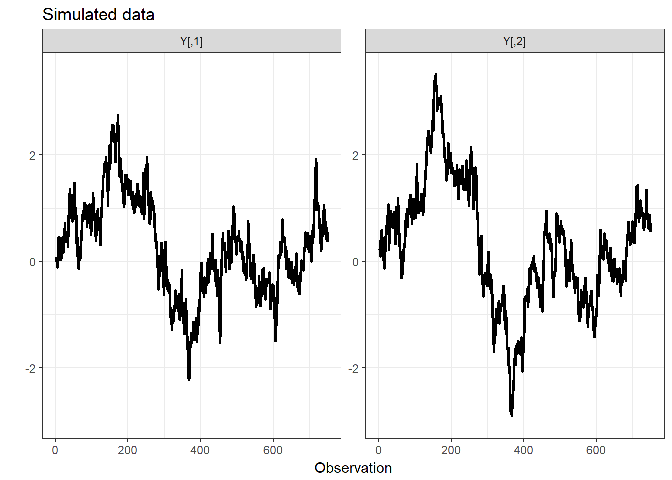
MS_VAR_example_sim.R
The first example file fits an unrestricted two-dimensional, two-state case of (1), with one autoregressive lag:
\[\begin{equation} \boldsymbol{Y}_{t} ={\boldsymbol{\phi}_1}_{(S_{t})}\boldsymbol{Y}_{t-1} +\boldsymbol{\mu}_{(S_{t})}+\boldsymbol{\epsilon}_{t},\qquad\boldsymbol{\epsilon}_{t}\sim\mathcal{N}\left(\boldsymbol{0},\boldsymbol{\Sigma}_{(S_{t})}\right),\qquad\boldsymbol{Y}_{t}\in\mathbb{R}^{2}. \end{equation}\]The data input is a simulated data set, generated by the file Data_generator.R in the repository.
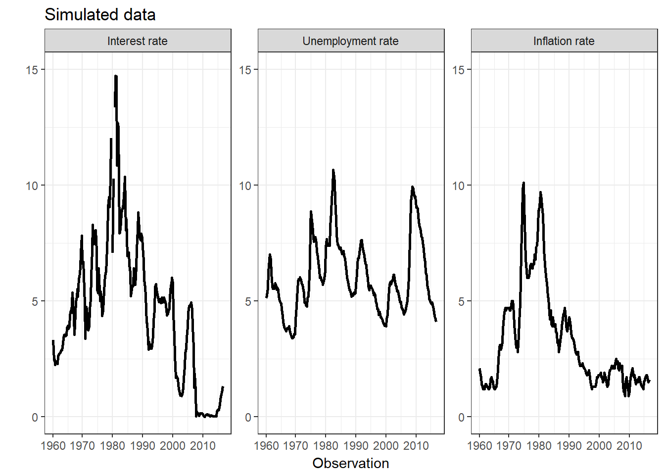
MS_VAR_example_USmacro.R
The second example file fits a three-dimensional, two-state case of (1), with four autoregressive lags, where the Markov-switching is restricted to the covariance structure: \[\begin{equation} \boldsymbol{Y}_{t} =\boldsymbol{\phi}_{1}\boldsymbol{Y}_{t-1}+\boldsymbol{\phi}_{2}\boldsymbol{Y}_{t-2}+\boldsymbol{\phi}_{3}\boldsymbol{Y}_{t-3}+\boldsymbol{\phi}_{4}\boldsymbol{Y}_{t-4}+\boldsymbol{\mu}+\boldsymbol{\epsilon}_{t},\qquad\boldsymbol{\epsilon}_{t}\sim\mathcal{N}\left(\boldsymbol{0},\boldsymbol{\Sigma}_{(S_{t})}\right),\qquad\boldsymbol{Y}_{t}\in\mathbb{R}^{3}. \end{equation}\]Following Lanne et al.(2010), the data input is a quarterly US macro data set, consisting of inflation, unemployment and an interest rate (3-Month Treasury Bill), ranging from January 1960 to January 2018. This data set is available in the repository.
Running the code
To be able to run the code, you should install R and Rstudio. After opening Rstudio, you need to install the following packages: rstan, coda and rstudioapi.
Then download the complete repository, keeping the original file structure. You should now be able to run one of the example files.
Below is some of the resulting output from the first example file, using 4 chains:
options(scipen=999) # avoid scientific notation
summary(pars_ls$pars)$statistics[1:pars_ls$index[1],]
## Mean SD Naive SE Time-series SE
## Q[1,1] 0.9691076593 0.010064709 0.00015913702 0.00013661482
## Q[2,2] 0.8767816057 0.039793706 0.00062919373 0.00052852579
## Q[1,2] 0.0308923407 0.010064709 0.00015913702 0.00013661482
## Q[2,1] 0.1232183943 0.039793706 0.00062919373 0.00052852579
## mu[1,1] 0.0060437427 0.007334371 0.00011596659 0.00008352485
## mu[2,1] 0.0303560824 0.025061662 0.00039625968 0.00028620366
## mu[1,2] 0.0009007403 0.007262776 0.00011483457 0.00008189346
## mu[2,2] 0.0172397612 0.027091917 0.00042836083 0.00032953087
## phi[1,1,1] 0.5874560258 0.031881257 0.00050408694 0.00050392536
## phi[2,1,1] 0.9276820980 0.046285310 0.00073183501 0.00068726288
## phi[1,2,1] -0.0678393937 0.031799041 0.00050278699 0.00050745179
## phi[2,2,1] 0.0852113837 0.045305205 0.00071633819 0.00069887113
## phi[1,1,2] 0.3052529153 0.023702753 0.00037477344 0.00038034655
## phi[2,1,2] 0.0391969647 0.040803556 0.00064516087 0.00061162543
## phi[1,2,2] 1.0418985187 0.024391420 0.00038566221 0.00039295457
## phi[2,2,2] 0.9016403627 0.042870930 0.00067784892 0.00064427269
## sigma[1,1,1] 0.0248701678 0.001670158 0.00002640752 0.00002048969
## sigma[2,1,1] 0.0718282467 0.010037321 0.00015870397 0.00013299935
## sigma[1,2,1] 0.0061532123 0.001136347 0.00001796723 0.00001404714
## sigma[2,2,1] 0.0015150417 0.006767256 0.00010699972 0.00008347834
## sigma[1,1,2] 0.0061532123 0.001136347 0.00001796723 0.00001404714
## sigma[2,1,2] 0.0015150417 0.006767256 0.00010699972 0.00008347834
## sigma[1,2,2] 0.0250218394 0.001632539 0.00002581270 0.00001916521
## sigma[2,2,2] 0.0696324964 0.009839120 0.00015557015 0.00012895136plot(pars_ls$pars[,c(1,pars_ls$index[2])])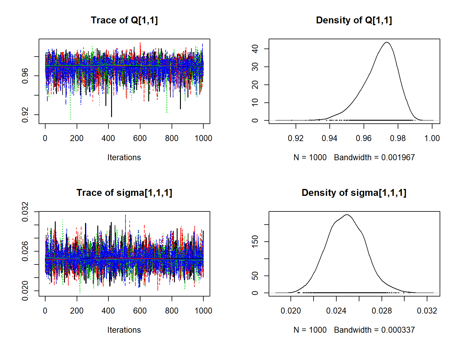
As the first example file uses simulated data, we can compare the estimated state values (black) to the actual states (red):
states=as.matrix(pars_ls$pars)[,(pars_ls$index[1]+1):pars_ls$index[3]]
plot(colMeans(states),ylab="Mean state",xlab="Observation")
points(S+1.01,col='red')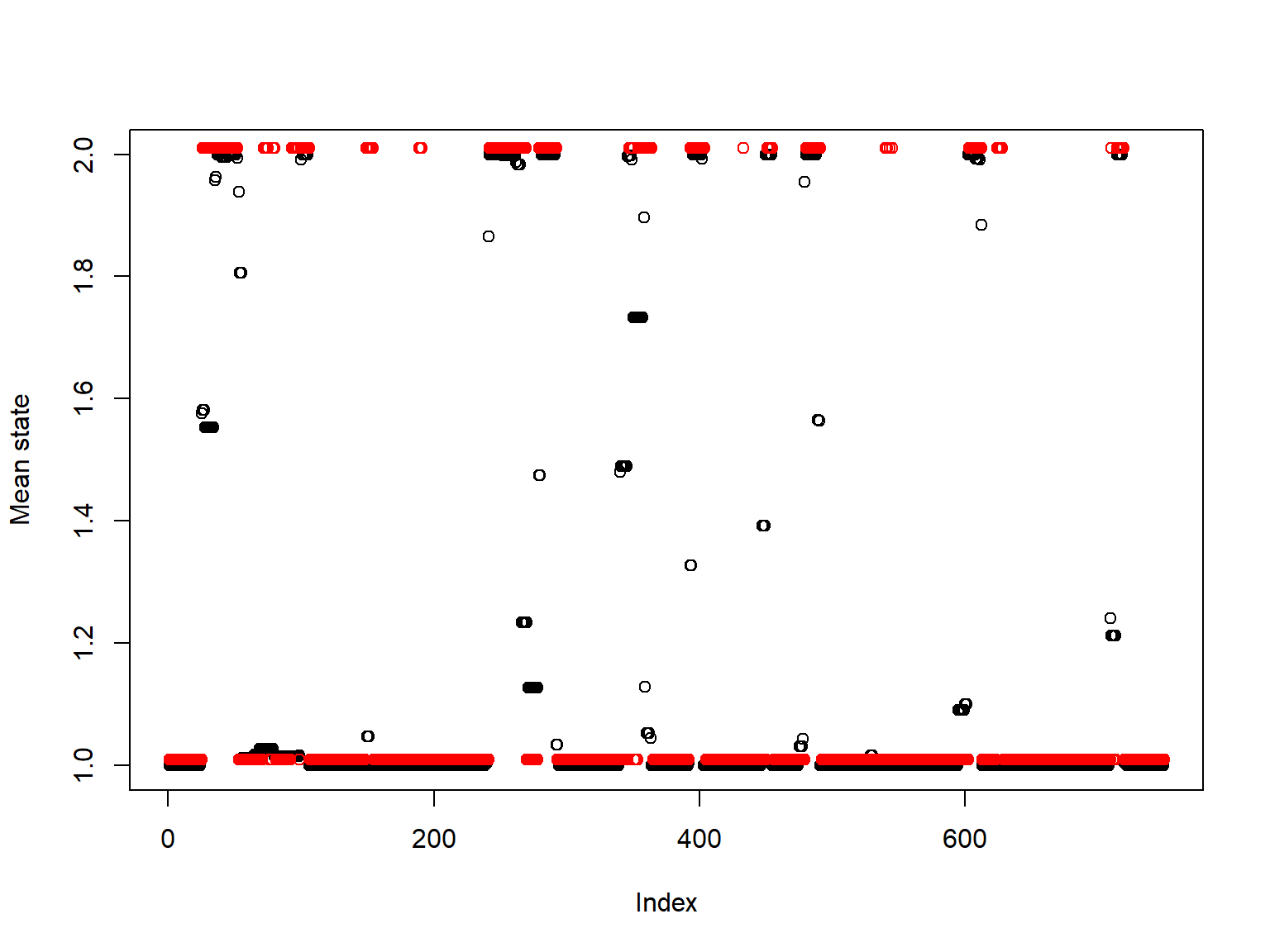
For details on parameter priors, model specification and label-switching, see the repository wiki.